Examples
Example 1: Max-cut
This is a polynomial optimization problem of commutative variables mentioned in Section 5.12 of Henrion et. al (2009). We rely on NumPy to remove the equality constraints from the problem
import numpy as np
W = np.diag(np.ones(8), 1) + np.diag(np.ones(7), 2) + np.diag([1, 1], 7) + \
    np.diag([1], 8)
W = W + W.T
n = len(W)
e = np.ones(n)
Q = (np.diag(np.dot(e.T, W)) - W) / 4

x = generate_variables('x', n)
equalities = [xi ** 2 - 1 for xi in x]

objective = -np.dot(x, np.dot(Q, np.transpose(x)))

sdp = SdpRelaxation(x)
sdp.get_relaxation(1, objective=objective, equalities=equalities,
                   removeequalities=True)
sdp.solve()
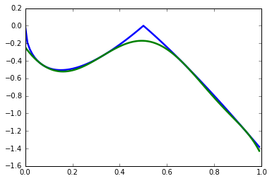
Example 2: Parametric Polynomial Optimization Problems
In a parametric polynomial optimization problem, we can separate two sets of variables, and one set acts as a parameter to the problem. More formally, we would like to find the following function:
where \(x\in\mathbf{X}=\{x\in \mathbb{R}^n: h_k(x)\geq 0, k=r+1,\ldots,t\}\). We can approximate \(J(x)\) using the dual an SDP relaxation. The following implements Example 4 from Lasserre (2010).
from math import sqrt
from sympy import integrate, N
import matplotlib.pyplot as plt

def J(x):
    return -2*abs(1-2*x)*sqrt(x/(1+x))

def Jk(x, coeffs):
    return sum(ci*x**i for i, ci in enumerate(coeffs))

level = 4
x = generate_variables('x')[0]
y = generate_variables('y', 2)
f = (1-2*x)*(y[0] + y[1])

gamma = [integrate(x**i, (x, 0, 1)) for i in range(1, 2*level+1)]
marginals = flatten([[x**i-N(gamma[i-1]), N(gamma[i-1])-x**i]
                    for i in range(1, 2*level+1)])

inequalities = [x*y[0]**2 + y[1]**2 - x,  - x*y[0]**2 - y[1]**2 + x,
                y[0]**2 + x*y[1]**2 - x,  - y[0]**2 - x*y[1]**2 + x,
                1-x, x]
sdp = SdpRelaxation(flatten([x, y]))
sdp.get_relaxation(level, objective=f, momentinequalities=marginals,
                   inequalities=inequalities)
sdp.solve()
coeffs = [sdp.extract_dual_value(0, range(len(inequalities)+1))]
coeffs += [sdp.y_mat[len(inequalities)+1+2*i][0][0] - sdp.y_mat[len(inequalities)+1+2*i+1][0][0]
           for i in range(len(marginals)//2)]

x_domain = [i/100. for i in range(100)]
plt.plot(x_domain, [J(xi) for xi in x_domain], linewidth=2.5)
plt.plot(x_domain, [Jk(xi, coeffs) for xi in x_domain], linewidth=2.5)
plt.show()
Example 3: Sparse Relaxation with Chordal Extension
This method replicates the behaviour of SparsePOP (Waki et. al, 2008). The following is a simple example:
level = 2
X = generate_variables('x', 3)

obj = X[1] - 2*X[0]*X[1] + X[1]*X[2]
inequalities = [1-X[0]**2-X[1]**2, 1-X[1]**2-X[2]**2]

sdp = SdpRelaxation(X)
sdp.get_relaxation(level, objective=obj, inequalities=inequalities,
                   chordal_extension=True)
sdp.solve()
print(sdp.primal, sdp.dual)
Example 4: Mixed-Level Relaxation of a Bell Inequality
It is often the case that moving to a higher-order relaxation is computationally prohibitive. For these cases, it is possible to inject extra monomials to a lower level relaxation. We refer to this case as a mixed-level relaxation.
As an example, we consider the CHSH inequality in the probability picture at level 1+AB relaxation. The lazy way of doing this is as follows:
level = 1
I = [[ 0,   -1,    0 ],
     [-1,    1,    1 ],
     [ 0,    1,   -1 ]]
print(maximum_violation(A_configuration, B_configuration, I, level,
      extra='AB')
This will immediately give you the negative of the maximum violation. The function maximum_violation only works for two-party configuration, so for educational purposes, we spell out what goes on in the background. With level and I defined as above, we create the measurements that will make up the probabilities, and define the objective function with the I matrix.
P = Probability([2, 2], [2, 2])
objective = define_objective_with_I(I, P)
Unfortunately, the function define_objective_with_I only works for two parties again, which is not surprising, as it would be hard to define an I matrix for more than two parties. So if you have a multipartite scenario, you can use the probabilities to define your Bell inequality. For the CHSH, it is
CHSH = -P([0],[0],'A') + P([0,0],[0,0])  + P([0,0],[0,1]) + \
        P([0,0],[1,0]) - P([0,0],[1,1]) - P([0],[0],'B')
Note that we can only minimize a function, so we have to flip the sign to get the same objective function as above:
objective = -CHSH
We need to generate the monomials we would like to add to the relaxation. This is aided by a helper function in the class Probability. We only need to provide the strings we would like to see – this time it is AB:
sdp = SdpRelaxation(P.get_all_operators())
sdp.get_relaxation(level, objective=objective,
                   substitutions=P.substitutions,
                   extramonomials=P.get_extra_monomials('AB'))
sdp.solve()
print(sdp.primal)
Example 5: Additional manipulation of the generated SDPs with PICOS
A compatibility layer with PICOS allows additional manipulations of the
optimization problem and also calling a wider ranger of solvers.
Assuming that the PICOS dependencies are in PYTHONPATH, we
can pass an argument to the function get_relaxation to generate a
PICOS optimization problem. Using the same example as before, we change
the relevant function call to:
P = sdp.convert_to_picos()
This returns a PICOS problem. For instance, we can manually define the value of certain elements of the moment matrix before solving the SDP:
X = P.get_variable('X')
P.add_constraint(X[0, 1] == 0.5)
Finally we can solve the SDP with any of solvers that PICOS supports:
P.solve()
Example 6: Bosonic System
The system Hamiltonian describes \(N\) harmonic oscillators with a parameter \(\omega\). It is the result of second quantization and it is subject to bosonic constraints on the ladder operators \(a_{k}\) and \(a_{k}^{\dagger}\) (see, for instance, Section 22.2 in M. Fayngold and Fayngold (2013)). The Hamiltonian is written as
Here \(^{\dagger}\) stands for the adjoint operation. The constraints on the ladder operators are given as
where \([.,.]\) stands for the commutation operator \([a,b]=ab-ba\).
Clearly, most of the constraints are monomial substitutions, except \([a_{i},a_{i}^{\dagger}]=1\), which needs to be defined as an equality. The Python code for generating the SDP relaxation is provided below. We set \(\omega=1\), and we also set Planck’s constant \(\hbar\) to one, to obtain numerical results that are easier to interpret.
from sympy.physics.quantum.dagger import Dagger

level = 1          # Level of relaxation
N = 4              # Number of variables
hbar, omega = 1, 1 # Parameters for the Hamiltonian

# Define ladder operators
a = generate_operators('a', N)

hamiltonian = sum(hbar*omega*(Dagger(ai)*ai+0.5) for ai in a)
substitutions = bosonic_constraints(a)

sdp = SdpRelaxation(a)
sdp.get_relaxation(level, objective=hamiltonian,
                   substitutions=substitutions)
sdp.solve()
The result is very close to two. The result is similarly precise for arbitrary numbers of oscillators.
It is remarkable that we get the correct value at the first level of relaxation, but this property is typical for bosonic systems (Navascués et al. 2013).
Example 7: Using the Nieto-Silleras Hierarchy
One of the newer approaches to the SDP relaxations takes all joint probabilities into consideration when looking for a maximum guessing probability, and not just the ones included in a particular Bell inequality (Nieto-Silleras, Pironio, and Silman 2014; Bancal, Sheridan, and Scarani 2014). Ncpol2sdpa can generate the respective hierarchy.
To deal with the joint probabilities necessary for setting constraints, we also rely on QuTiP (Johansson, Nation, and Nori 2013):
from math import sqrt
from qutip import tensor, basis, sigmax, sigmay, expect, qeye
We will work in a CHSH scenario where we are trying to find the maximum guessing probability of the first projector of Alice’s first measurement. We generate the joint probability distribution on the maximally entangled state with the measurements that give the maximum quantum violation of the CHSH inequality:
psi = (tensor(basis(2,0),basis(2,0)) + tensor(basis(2,1),basis(2,1))).unit()
A = [(qeye(2) + sigmax())/2, (qeye(2) + sigmay())/2]
B = [(qeye(2) + (-sigmay()+sigmax())/sqrt(2))/2,
     (qeye(2) + (sigmay()+sigmax())/sqrt(2))/2]
Next we need the basic configuration of the probabilities and we must make them match the observed distribution.
P = Probability([2, 2], [2, 2])
behaviour_constraints = [
  P([0],[0],'A')-expect(tensor(A[0], qeye(2)), psi),
  P([0],[1],'A')-expect(tensor(A[1], qeye(2)), psi),
  P([0],[0],'B')-expect(tensor(qeye(2), B[0]), psi),
  P([0],[1],'B')-expect(tensor(qeye(2), B[1]), psi),
  P([0,0],[0,0])-expect(tensor(A[0], B[0]), psi),
  P([0,0],[0,1])-expect(tensor(A[0], B[1]), psi),
  P([0,0],[1,0])-expect(tensor(A[1], B[0]), psi),
  P([0,0],[1,1])-expect(tensor(A[1], B[1]), psi)]
We also have to define normalization of the subalgebras, in this case, only one:
behaviour_constraints.append("-0[0,0]+1.0")
From here, the solution follows the usual pathway:
level = 1
sdp = SdpRelaxation(P.get_all_operators(), normalized=False, verbose=1)
sdp.get_relaxation(level, objective=-P([0],[0],'A'),
                   momentequalities=behaviour_constraints,
                   substitutions=P.substitutions)
sdp.solve()
print(sdp.primal, sdp.dual)
Example 8: Using the Moroder Hierarchy
This type of hierarchy allows for a wider range of constraints of the optimization problems, including ones that are not of polynomial form (Moroder et al. 2013). These constraints are hard to impose using SymPy and the sparse structures in Ncpol2Sdpa. For this reason, we separate two steps: generating the SDP and post-processing the SDP to impose extra constraints. This second step can be done in MATLAB, for instance.
Then we set up the problem with specifically with the CHSH inequality in the probability picture as the objective function. This part is identical to the one discussed in Section [mixedlevel].
I = [[ 0,   -1,    0 ],
     [-1,    1,    1 ],
     [ 0,    1,   -1 ]]
P = Probability([2, 2], [2, 2])
objective = define_objective_with_I(I, P)
When obtaining the relaxation for this kind of problem, it can prove useful to disable the normalization of the top-left element of the moment matrix. Naturally, before solving the problem this should be set to zero, but further processing of the SDP matrix can be easier without this constraint set a priori. Hence we write:
level = 1
sdp = MoroderHierarchy([flatten(P.parties[0]), flatten(P.parties[1])],
                       verbose=1, normalized=False)
sdp.get_relaxation(level, objective=objective,
                   substitutions=P.substitutions)
We can further process the moment matrix, for instance, to impose partial positivity, or a matrix decomposition. To do these operations, we rely on PICOS:
Problem = sdp.convert_to_picos(duplicate_moment_matrix=True)
X = Problem.get_variable('X')
Y = Problem.get_variable('Y')
Z = Problem.add_variable('Z', (sdp.block_struct[0],
                         sdp.block_struct[0]))
Problem.add_constraint(Y.partial_transpose()>>0)
Problem.add_constraint(Z.partial_transpose()>>0)
Problem.add_constraint(X - Y + Z == 0)
Problem.add_constraint(Z[0,0] == 1)
solution = Problem.solve()
print(solution)
Alternatively, with SeDuMi’s fromsdpa function (Sturm 1999), we can also impose the positivity of the partial trace of the moment matrix using MATLAB, or decompose the moment matrix in various forms. For this, we have to write the relaxation to a file:
sdp.write_to_file("chsh-moroder.dat-s")
If all we need is the partial positivity of the moment matrix, that is actually nothing but an extra symmetry. We can request this condition by passing an argument to the constructor, leading to a sparser SDP:
sdp = MoroderHierarchy([flatten(P.parties[0]), flatten(P.parties[1])],
                       verbose=1, ppt=True)
sdp.get_relaxation(level, objective=objective,
                   substitutions=P.substitutions)
References
Bancal, J.D., L. Sheridan, and V. Scarani. 2014. “More Randomness from the Same Data.” New Journal of Physics 16 (3): 033011. doi:10.1088/1367-2630/16/3/033011.
Fayngold, M., and V. Fayngold. 2013. Quantum Mechanics and Quantum Information. Wiley-VCH.
Henrion, D., J. Lasserre and J. Löfberg. 2009. “GloptiPoly 3: Moments, Optimization and Semidefinite Programming.” Optimization Methods & Software, 24: 761–779.
Johansson, J.R., P.D. Nation, and Franco Nori. 2013. “QuTiP 2: A Python Framework for the Dynamics of Open Quantum Systems.” Computer Physics Communications 184 (4): 1234–40. doi:10.1016/j.cpc.2012.11.019.
Lasserre, J. B. 2010. “A Joint+Marginal Approach to Parametric Polynomial Optimization.” SIAM Journal on Optimization 20(4):1995–2022. doi:10.1137/090759240.
Moroder, Tobias, Jean-Daniel Bancal, Yeong-Cherng Liang, Martin Hofmann, and Otfried Gühne. 2013. “Device-Independent Entanglement Quantification and Related Applications.” Physics Review Letters 111 (3). American Physical Society: 030501. doi:10.1103/PhysRevLett.111.030501.
Navascués, M., A. García-Sáez, A. Acín, S. Pironio, and M.B. Plenio. 2013. “A Paradox in Bosonic Energy Computations via Semidefinite Programming Relaxations.” New Journal of Physics 15 (2): 023026. doi:10.1088/1367-2630/15/2/023026.
Nieto-Silleras, O., S. Pironio, and J. Silman. 2014. “Using Complete Measurement Statistics for Optimal Device-Independent Randomness Evaluation.” New Journal of Physics 16 (1): 013035. doi:10.1088/1367-2630/16/1/013035.
Pironio, S., M. Navascués, and A. Acín. 2010. “Convergent Relaxations of Polynomial Optimization Problems with Noncommuting Variables.” SIAM Journal on Optimization 20 (5). SIAM: 2157–80. doi:10.1137/090760155.
Sturm, J.F. 1999. “Using SeDuMi 1.02, a MATLAB Toolbox for Optimization over Symmetric Cones.” Optimization Methods and Software 11 (1-4): 625–53.
Waki, H.; S. Kim, M. Kojima, M. Muramatsu, and H. Sugimoto. 2008. “Algorithm 883: SparsePOP—A Sparse Semidefinite Programming Relaxation of Polynomial Optimization Problems.” ACM Transactions on Mathematical Software, 2008, 35(2), 15. doi:10.1145/1377612.1377619.
Yamashita, M., K. Fujisawa, and M. Kojima. 2003. “SDPARA: Semidefinite Programming Algorithm Parallel Version.” Parallel Computing 29 (8): 1053–67.